Microsoft Excel offers a lot of formatting options so that you can properly format the data in your cells. So if you want to learn how to show a dollar sign next to numbers in Excel, then it’s possible to do so with currency formatting.
It’s very common for Excel users to create spreadsheets that include values for money. Whether it’s for business purposes or simply trying to track your personal expenses, Excel is a helpful tool for that sort of data. Master Your Tech offers a variety of different guides to help you work with Excdel in additional ways.
You can format any information that you enter into your cells in a lot of different manners, including setting that information as currency. You can also choose to show a dollar sign next to currency values to make them easier to identify.
Our guide below is going to show you how to display a number sign next to numbers in Excel.
How to Show A Dollar Sign Next to Numbers in Excel for Office 365
- Open your spreadsheet.
- Select the cells to change.
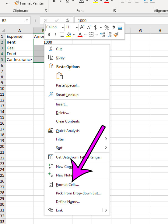
- Right-click on a selected cell and choose Format Cells.
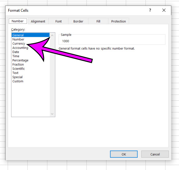
- Click Currency.
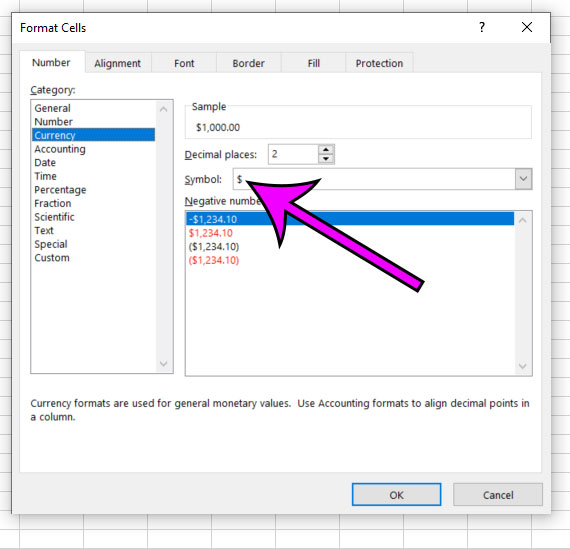
- Click the Symbol dropdown and choose the dollar sign.
- Click OK.
Our guide continues below with additional information on showing a dollar sign next to numbers in Excel, including pictures of these steps.
How to Format Numbers with a Dollar Sign in Excel
The steps in this article were performed in the Microsoft Excel for Office 365 version of the application, but will also work in most other versions of Excel.
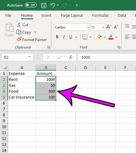
Step 1: Open the Excel file containing the cells that you want to format.
Step 2: Select the cell or cells to which you wish to apply this formatting.
You can select an entire row by clicking the row number at the left side of the window, or you can select an entire column by clicking the column letter at the top.
Step 3: Right-click on a selected cell, then choose the Format Cells option at the bottom of the menu.
Step 4: Click the Currency option from the column at the left side of the window.
Step 5: Click the dropdown menu to the right of Symbol, then choose the dollar sign option.
Note that the $ is probably selected by default, so you may not need to do anything here.
Step 6: Click the OK button to apply the change.
You can also change the formatting for a selection by clicking the Home tab at the top of the window, then clicking the dropdown menu in the Number section of the ribbon and specifying your options there.
Find out how to remove gridlines in Excel if you don’t want to see lines on your screen or when you print your document.
Matthew Simpson has been creating online tutorial for computers and smartphones since 2010. His work has been read millions of times and helped people to solve a number of various tech problems. His specialties include Windows, iPhones, and Google apps.